This article provides a tutorial on how to create an S-Curve with earned value metrics in Tableau using data from an Excel workbook. The article walks through the ETL process using R code, visualizing cost estimates and project progress indicators, and building the S-Curve to project future costs and completion times. The S-Curve is created by calculating the Estimate at Completion (EAC) and plotting it against actual and earned values over time. The software used for project controls is Dash360.
Creating an S-Curve with R & Tableau
Displaying an Scurve with Earned Value Metrics in Tableau for data visualization and interactive adjustment
Data Source
For this exercise we are using Excel workbooks as the source of the analysis.
Although each data extract contains 15+ columns and calculations, for this exercise, we’re going to focus only on the following features:
- Cost Classes – Strings (Actuals | Budget | Earned | Forecast)
- WBS – String (Work Breakdown Structure)
- Resource Type – String (labor | nonlabor | travel)
- Resource Date – Date
- Fiscal Year – Integer
- Item Cost (or Value) – Numeric
Extraction, Transform and Load (ETL) process
The extracted data contains information for actuals, budget, earned value, and forecast numbers. All four cost categories follow the same structure and are recorded at the activity level. That means, for the same activity, multiple records can be stored in the tool; one for each cost category.
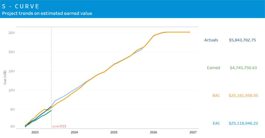
We can leverage the following R code (image #1) to merge the two files, but more generally, we can continue to add any additional extracts into the folder specified and use this function to append at any extent.
Some callouts from the R code:
- The dir_files variable will contain all files from the folder specified in the path. Make sure to keep only the files that you are going to use in the analysis.
- The data_transform function is specific for this project, as there are some transformations made to the raw data.
- The ETL process follows a very simple iteration for every file in the data directory: read into R, transform, and append.
Image #1: R Code
Visualizing an S-Curve for project performance
Now that we have a single source of truth (SSOT) from the ETL process, we can start constructing the different EVM concepts. For this exercise, we’re using Tableau as the primary visualization tool.
1. Cost estimates
We’ll start with the high-level cost classes to identify and validate our data against the project’s performance by adding the cost category by fiscal year (image #2). We need to make sure we’re collecting what we planned – or budget, what has been done – or earned value, and how much we have spent – or actual cost, before we start evaluating further.
Simply drag the cost class variable into “Columns”, fiscal year into “Rows”, and item_cost (or Value) into “Text” box.
Note: Make sure the year is set as discrete
We can now easily identify cost estimates as Actuals, Budget, Earned, and Forecast by any breakdown needed.
2. Project’s progress indicators
To assess the project’s progress, we need to measure how far or ahead we’re at in reference to the budget and schedule. To accomplish this, we’ll use the following calculations:
- Cost Variance (CV)=Earned Value (EV)-Actual Cost (AC)
- Schedule Variance (SV)=Earned Value (EV)-Planned Value (PV)
- Cost Performance Index (CPI)=(Earned Value (EV))/(Actual Cost (AC))
- Schedule Performance Index (SPI)=(Earned Value (EV))/(Planned Value (PV))
Both CV and SV – and so the CPI and SPI – help us determine whether the project is going in the right direction or not. More generally, if our actual cost is coherent with what we have achieved so far; and if what we planned is being met.
Similarly, as in the previous visualization, using calculated fields in Tableau we can picture the project’s progress.
Calculated Field #1 to #3 – Cost Class
- Repeat for Actual, Earned, and Budget.
Actual
IF [Cost Class] = 'Actual'
THEN [Item Cost]
END
Calculated Field #4 to #7 – Project’s progress
CV
SUM([Earned]) – SUM([Actual])
SV
SUM([Earned]) – SUM([Budget])
CPI
SUM([Earned]) / SUM([Actual])
SPI
SUM([Earned]) / SUM([Actual])
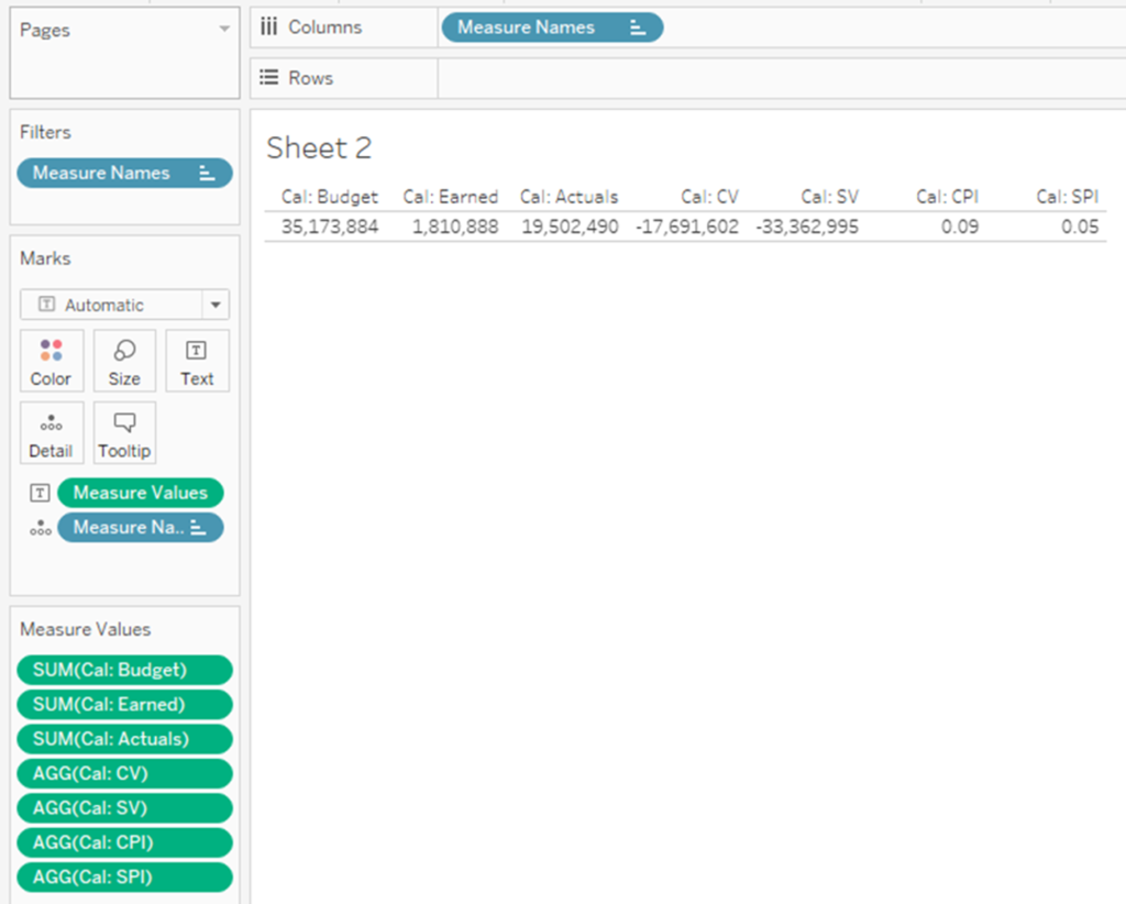
After creating the four calculated fields using the formulas above, simply drag the Measure Values into the “Text” box, and Measure Names into “Columns” or “Rows”. Filter the Measure Names to only show the desired calculations and format accordingly (image #3).
Image #3: Project progress
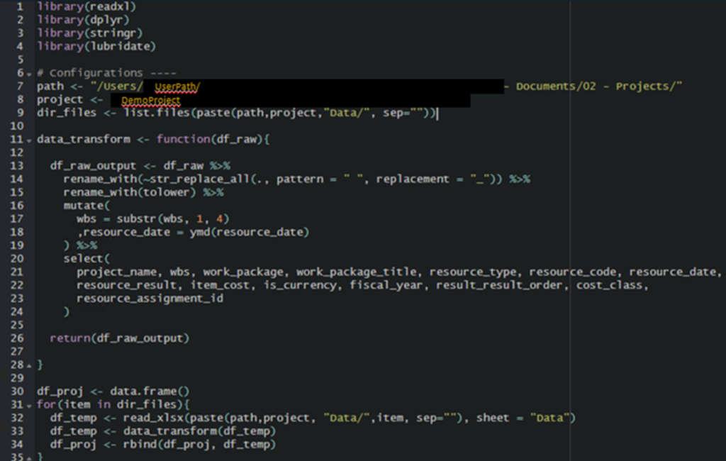
3. Project estimations & S-Curve
Now that we have calculated the cost estimates and the project’s progress, we can start building the S-Curve. An S-Curve in the EVM context will plot the project’s development in time and will give us information about the future of the project and completion times.
To understand what the estimates at completion are, we will need to use the EAC calculation:
- Estimate at Completion (EAC)=PV-EV+AC
- Calculated based on Planned Value and Earned Value.
The total Estimate At Completion will give us an indication on how far away are we from our target date and planned cost.
To do that, we’re going to use the following parameters and calculated fields:
Parameter #1 – Report Date
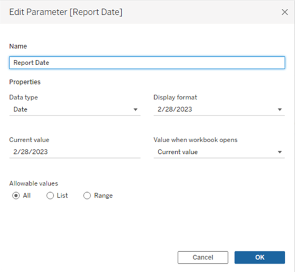
This date can be set to the current date or for a specific report in time.
Calculated Field #8 to #11 – Running cost up to report date
- Repeat for Actual, Earned, Budget, and Forecast.
Actual Running
IF
(ATTR([Resource Date]) > [Report Date] AND SUM([Actual]) > 0)
OR ATTR([Resource Date]) <= [Report Date]
THEN RUNNING_SUM(SUM([Actual]))
ELSE NULL
END
Calculated Field #12 to #13 – Cost estimates at Complete
- Repeat for Actual and Earned.
AAC (Running)
RUNNING_SUM(SUM([Actual]))
Calculated Field #14 – Estimate at Complete (Running)
EAC (Running)
IF ATTR([Resource Date1]) <= [Report Date]THEN [Cal: Actuals (Running)]ELSE [Cal: Forecast (Running)]END
Calculated Field #15 – Has Budget – Only captures dates up to where budget is available
Has Budget
[Resource Date] <=
{
FIXED [Resource Result], [Resource Type], [Wbs]
:
MAX(IF [Cost Class] = 'Budget' THEN [Resource Date] END)
}
To build the S-Curve make sure to follow these steps:
- Drag Has Budget into filters. Only check “True”.
- Drag Resource Date into “Columns”. Make sure to have a continuous MONTH measure.
- Drag Measure Values into “Rows”. Edit the Measure Names filter to include only
- Actuals (Running)
- Earned (Running)
- Forecast (Running)
- Drag EAC (Running) into “Rows”, next to Measure Values.
- Right click on EAC (Running) and select “Dual Axis”.
- On the chart below, right click the EAC (Running) Y-axis and select “Synchronize Axis”.
- Drag Measure Names into “Color” box for both Measure Values and EAC (Running) in the Marks box.
After some editing and formatting you should end up with something like this: